Masking #

Prompt: Implement a kinegram and some moiré patterns which are close related visual phenomena to masking.

Visual masking is the reduction or elimination of the visibility of one brief (≤ 50 ms) stimulus, called the “target”, by the presentation of a second brief stimulus, called the “mask”. Introduced near the end of the 19th and beginning of the 20th century (Exner, 1868; McDougal, 1904; Sherrington, 1897; Stigler, 1911) and extensively studied since then, masking, an interesting phenomenon in its own right, is a useful tool for exploring the dynamics of visual information processing (Breitmeyer & Öğmen, 2006). As a technique for studying the dynamic and microgenetic aspects of vision Visual Masking.

Kinegram #

Visual artist Gianni A. Sarcone has produced animations that he calls kinegrams since 1997. He describes his animations as “optic kinetic media” that “artfully combine the visual effects of moiré patterns with the zoetrope animation technique”. Sarcone also created rotating animations that use a transparent disc with radial lines that has to be spun around its center to animate the picture Kinegram

Implementation #

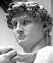
In the following image there is a background image that is composed of a wolf main shape, but the figures that represent the wolf legs are incomplete and superimposed to allow a grid in movement to create the illusion of movement. Deepening in the code it was just required create multiple vertical lines and add an xOffset depending of the selected speed.

Kinegram

let startButton, stopButton;
let xOffset, xSpeed;
let img;

function preload() {
 img = loadImage('/showcase/lobo.jpg');
}

function setup() {
 createCanvas(700, 400);
 text = createP("Speed");
 startButton = createButton('Start');
 startButton.mousePressed(startGrid);
 stopButton = createButton('Stop');
 stopButton.mousePressed(stopGrid);
 input = createInput();
 input.value(2.5);
 startGrid();
}

function draw() {
 background(img);
 if (xOffset) {
   xOffset += xSpeed;
   if (xOffset > width) {
     xOffset = -width;
   }
 }
 drawLines();
}

function drawLines() {
 stroke(0);
 strokeWeight(5);
 let lineSpacing = 10;
 for (let x = -width*1000; x < width*1000; x += lineSpacing) {
   line(x + xOffset, 0, x + xOffset, height);
 }
}

function startGrid() {
 let val = input.value();
 xSpeed = parseFloat(val);
 xOffset = -width;
}

function stopGrid() {
 xOffset = null;
}

Moire Pattern #

Moire patterns are large-scale interference patterns that can be produced when a partially opaque ruled pattern with transparent gaps is overlaid on another similar pattern. For the moiré interference pattern to appear, the two patterns must not be completely identical, but rather displaced, rotated, or have slightly different pitch. Moiré pattern

Implementation #

In the first moire pattern were used mutiple circles and squares separated by an input parameter and multiplied by another parameter, the shapes are rotating endlessly and the dynamic intersection of the shapes create multiple figures along the created intersections sets.

In the second implemented moire pattern we use traingles and rectangles in the same way as the first pattern. Each pattern has two inputs, the first is the number of shapes to print and the second is the size of the shapes.

Moire Pattern 1

let figuresCount = 100;
let shapeSize = 4;

function setup() {
 createCanvas(400, 400);
 shapesCount = createInput(figuresCount);
 shapesCount.value(100);

 shapeSizesInput = createInput(shapeSize);
 shapeSizesInput.value(10);

 shapesCount.input(() => {
   figuresCount = parseInt(shapesCount.value());
 });

 shapeSizesInput.input(() => {
   shapeSize = parseInt(shapeSizesInput.value());
 });

}

let rotationAngle = 0;

function draw() {
 background(220);
 noFill();
 strokeWeight(2);

 
 for (let i = 0; i < figuresCount; i++) {
   let squareW = shapeSize * (figuresCount - i);

   rotate(radians(rotationAngle)); 
   stroke("black");
   rectMode(CENTER);
   rect(-squareW/2, -squareW/2, squareW, squareW); 
   rect(-squareW/3, -squareW/3, squareW, squareW); 
 }
 
 rotationAngle += 1/5; 
}

Moire Pattern 2

let numShapes = 100;
let shapeSize = 10;
let angle = 0;

function setup() {
 createCanvas(400, 400);
 numShapesInput = createInput(numShapes);
 numShapesInput.value(100);

 shapeSizesInput = createInput(shapeSize);
 shapeSizesInput.value(10);

 numShapesInput.input(() => {
   numShapes = parseInt(numShapesInput.value());
 });

 shapeSizesInput.input(() => {
   shapeSize = parseInt(shapeSizesInput.value());
 });
}

function draw() {
 background(220);
 noFill();

 // Center the shapes in the canvas
 let centerX = width / 2;
 let centerY = height / 2;

 // Draw a loop of triangles
 stroke("black");
 for (let i = 0; i < numShapes; i++) {
   let triangleX = centerX;
   let triangleY = centerY;
   let triangleR = shapeSize * (numShapes - i);
   let triangleA = angle + i * (360 / numShapes);
   push();
   translate(triangleX, triangleY);
   rotate(radians(triangleA));
   triangle(0, 0, triangleR, triangleR * sqrt(3) / 2, -triangleR, triangleR * sqrt(3) / 2);
   pop();
 }

 // Draw a loop of squares
 stroke("black");
 for (let i = 0; i < numShapes; i++) {
   let squareX = centerX;
   let squareY = centerY;
   let squareW = shapeSize * (numShapes - i);
   let squareA = angle - i * (360 / numShapes);
   push();
   translate(squareX, squareY);
   rotate(radians(squareA));
   rectMode(CENTER);
   rect(0, 0, squareW, squareW);
   pop();
 }

 angle += 1;
}

Floyd-Steinberg dithering #

Prompt: Implement a color mapping application that helps people who are color blind see the colors around them.

Dithering is, a it´s core, a form of noise that is applied to a medium (either sound or an image) and it´s used to prevent certain color problems when used in image processing or as a means to compress audio. Image od David using dithering Dithering in image processing can be achieved by many different ways, but in this case we´re focusing on the Floyd-Steinberg algorithm for image dithering. To understand this algorithm fyllu it is necessary to break it in a couple of portions:

Quantizing #

Quantizing in the image processing scope, is a process in wich the image is divided into individual pixels and each and every one of them is filtered through their respective red, green and blue channels. But first it´s necessary to trace every pixel´s position in the image, a helpfull way to think about it is like a grid of pixels, where every pixel has a (x,y) location to it:

0	1	2	3
1	x	x	x
2	x	x	x
3	x	x	x

Now, after every pixel has it´s coordinates we can filter every individual pixel through every color channel limiting the available number of colors it can take: For example, if we take an RGB color as a number between 0 and 255, if we limit the colors to only two 0 or 255 (black and white), if a color value on any channel is les than 127, the pixel will round down to 0 and it´ll take the color black. On the other hand, if the value is greater than 127, the pixel will round up to 255 and take the color white. This very thing happens if the color spectrum goes from 2 possibilities to 5, or 125, etc.

There´s something to keep in mind, every time dithering is applied to an image there´s an error that is being generated. This error can be used and spread through the pixel´s neighbours to have a more detailed image withoud much fidelity loss.

Quantizing error #

To quantize the error and incorporate it into the the image processing, first we just need to do a simple substraction. The operation consists of substracting the original value of the color channel from the quantized value , the result is the error_ Image od David using dithering Now, finnaly it´s time for the Floyd-Steinberg algorithm.

Floyd-Steinberg algorithm #

This algorithm focuses on “streching” or dispersing the error to the neighboring pixels, this is achieved by the use of this small pseudo-code and better explaine by this graph:

	pixels[_x_ + 1][_y_    ] := pixels[_x_ + 1][_y_    ] + quant_error × 7 / 16
	pixels[_x_ - 1][_y_ + 1] := pixels[_x_ - 1][_y_ + 1] + quant_error × 3 / 16
    pixels[_x_    ][_y_ + 1] := pixels[_x_    ][_y_ + 1] + quant_error × 5 / 16
    pixels[_x_ + 1][_y_ + 1] := pixels[_x_ + 1][_y_ + 1] + quant_error × 1 / 16

Image od David using dithering

Here the error “spreads” in different directions with different rates, thats why the pixel indexing was so important.

After having the quantized error calculated and embeded into the algorithm it´s time to put back all the pixels and reveal the waited result!

Floyd-Steinberg dithering #

Prompt: Implement a color mapping application that helps people who are color blind see the colors around them.

Quantizing #

0	1	2	3
1	x	x	x
2	x	x	x
3	x	x	x

Quantizing error #

Floyd-Steinberg algorithm #

This algorithm focuses on “streching” or dispersing the error to the neighboring pixels, this is achieved by the use of this small pseudo-code and better explaine by this graph:

	pixels[_x_ + 1][_y_    ] := pixels[_x_ + 1][_y_    ] + quant_error × 7 / 16
	pixels[_x_ - 1][_y_ + 1] := pixels[_x_ - 1][_y_ + 1] + quant_error × 3 / 16
    pixels[_x_    ][_y_ + 1] := pixels[_x_    ][_y_ + 1] + quant_error × 5 / 16
    pixels[_x_ + 1][_y_ + 1] := pixels[_x_ + 1][_y_ + 1] + quant_error × 1 / 16

Image od David using dithering

Here the error “spreads” in different directions with different rates, thats why the pixel indexing was so important.

After having the quantized error calculated and embeded into the algorithm it´s time to put back all the pixels and reveal the waited result!

Web app #

Prompt: Implement in software an image processing web app supporting different image kernels and supporting:

Image histogram visualization.
Different lightness (coloring brightness) tools.

On this exercise we provide a script to process images that can be embeded on any web application. But for practical purposes we show an example with predefined images.

The next p5 script allow us to load an image from our computer, then generates the histogram for the image and finally one can choose from various processes that can be applied to that image, when a process is applied the resulting image is automatically downloaded.

web-app.js

let HW = 400;
let HH = 400;
let HP = 200;
let BG = 8;

function drawRGBHistogram(imgBuffer) {
 let histR = (new Array(256)).fill(0);
 let histG = (new Array(256)).fill(0);
 let histB = (new Array(256)).fill(0);
 let maxB = 0;
 for (let i = 0; i < imgBuffer.length; i += 4) {
   histR[imgBuffer[i]]++;
   histG[imgBuffer[i + 1]]++;
   histB[imgBuffer[i + 2]]++;
 }

 maxB = Math.max(Math.max(...histR), Math.max(...histG), Math.max(...histB));

 const y1 = HP + HH;
 const dx = HW / 255;
 const dy = HW / maxB;
 rect(0, HP, HW, HH);
 strokeWeight(dx);
   
 for (let i = 0; i < 256; i++) {
   let x = i * dx;
   stroke(color(220,0,0,128));
   line(x, y1, x, y1 - histR[i] * dy);
   stroke(color(0,210,0,128));
   line(x, y1, x, y1 - histG[i] * dy);
   stroke(color(0,0,255,128));
   line(x, y1, x, y1 - histB[i] * dy);
   stroke(color(i, i, i));
   line(x, y1, x, y1 + BG);
 }
}

function drawBrightnessHistogram(imgBuffer) {
 let hist = (new Array(256)).fill(0);
 let maxB = 0;

 for (let i = 0; i < imgBuffer.length; i++) {
   // Ignoring alpha
   if (i%4 != 3) {
     hist[imgBuffer[i]]++;
   }
 }

 maxB = Math.max(...hist);

 const y1 = HP + HH;
 const dx = HW / 255;
 const dy = HW / maxB;
 rect(0, HP, HW, HH);
 strokeWeight(dx);
   
 for (let i = 0; i < 256; i++) {
   let x = i * dx;
   stroke(color("black"));
   line(x, y1 + BG, x, y1 - hist[i] * dy);
   stroke(color(i, i, i));
   line(x, y1, x, y1 + BG);
 }
}

function copyArray(a) {
 c = Array(a.length); 
 i = a.length;
 while(i--) c[i] = a[i];
 return a;
}

function applyLuma(){
 let lumaImg = createImage(img.width, img.height);
 lumaImg.loadPixels();
 for (let i = 0; i < img.pixels.length; i+=4) {
   lumaImg.pixels[i] = (img.pixels[i] + img.pixels[i + 1] + img.pixels[i + 2]) / 3;
   lumaImg.pixels[i + 1] = (img.pixels[i] + img.pixels[i + 1] + img.pixels[i + 2]) / 3;
   lumaImg.pixels[i + 2] = (img.pixels[i] + img.pixels[i + 1] + img.pixels[i + 2]) / 3;
   lumaImg.pixels[i + 3] = 255;
 }
 lumaImg.updatePixels();
 lumaImg.save('luma', 'png');
}

function convolve(name, matrix) {
 let convolvedImage = createImage(img.width, img.height);
 convolvedImage.loadPixels();
 for (let x = 0; x < img.width; x++) {
   for (let y = 0; y < img.height; y++) {
     let c = convolution(x, y, matrix, img);
     
     let loc = (x + y * img.width) * 4;
     convolvedImage.pixels[loc] = red(c);
     convolvedImage.pixels[loc + 1] = green(c);
     convolvedImage.pixels[loc + 2] = blue(c);
     convolvedImage.pixels[loc + 3] = alpha(c);
   }
 }
 convolvedImage.updatePixels();
 convolvedImage.save(name, 'png');
}

function convolution(x, y, matrix) {
 let rtotal = 0.0;
 let gtotal = 0.0;
 let btotal = 0.0;
 const offset = Math.floor(matrix.length / 2);
 for (let i = 0; i < matrix.length; i++){
   for (let j = 0; j < matrix.length; j++){
     
     // What pixel are we testing
     const xloc = (x + i - offset);
     const yloc = (y + j - offset);
     let loc = (xloc + yloc * img.width) * 4;

     // Make sure we haven't walked off our image, we could do better here
     loc = constrain(loc, 0 , img.pixels.length - 1);

     // Calculate the convolution
     // retrieve RGB values
     rtotal += (img.pixels[loc]) * matrix[i][j];
     gtotal += (img.pixels[loc + 1]) * matrix[i][j];
     btotal += (img.pixels[loc + 2]) * matrix[i][j];
   }
 }
 // Make sure RGB is within range
 rtotal = constrain(rtotal, 0, 255);
 gtotal = constrain(gtotal, 0, 255);
 btotal = constrain(btotal, 0, 255);
 
 // Return the resulting color
 return color(rtotal, gtotal, btotal);
}

function applySharpen() {
 convolve("Sharpen", kernels["Sharpen"]);
}

function applyBoxBlur() {
 convolve("BoxBlur", kernels["BoxBlur"]);
}

function applyGaussianBlur3x3() {
 convolve("GaussianBlur3x3", kernels["GaussianBlur3x3"]);
}

function applyGaussianBlur5x5() {
 convolve("GaussianBlur5x5", kernels["GaussianBlur5x5"]);
}

function applyUnsharp5x5() {
 convolve("Unsharp5x5", kernels["Unsharp5x5"]);
}

let kernels = {
 "Sharpen" : [[0,-1,0],
              [-1,5,-1],
              [0,-1,0]],
 "BoxBlur" : [[1/9,1/9,1/9],
               [1/9,1/9,1/9],
               [1/9,1/9,1/9]],
 "GaussianBlur3x3" : [[1/16,1/8,1/16],
                          [1/8,1/4,1/8],
                          [1/16,1/8,1/16]],
 "GaussianBlur5x5" : [[1/256,4/256,6/256,4/256,1/256],
                          [4/256,16/256,1/256,16/256,4/256],
                          [6/256,24/256,36/256,24/256,6/256],
                          [4/256,16/256,1/256,16/256,4/256],
                          [1/256,4/256,6/256,4/256,1/256]],
 "Unsharp5x5" : [[-1/256,-4/256,-6/256,-4/256,-1/256],
                            [-4/256,-16/256,-1/256,-16/256,-4/256],
                            [-6/256,-24/256,476/256,-24/256,-6/256],
                            [-4/256,-16/256,-1/256,-16/256,-4/256],
                            [-1/256,-4/256,-6/256,-4/256,-1/256]],
};

let img;
let input;
let histogramTypeSelect;
let sharpenButton;
let boxBlurButton;
let gaussianBlur3x3Button;
let gaussianBlur5x5Button;
let unsharpMasking5x5Button;
let lumaButton;


function handleFiles() {
 const fileList = this.files; /* now you can work with the file list */
 const file = fileList[0]

 var reader = new FileReader();

 reader.onload = function(e) {
   if (file.type === 'image/png' || file.type === 'image/jpeg') {
     img = loadImage(e.target.result, '');
     img.loadPixels();
   } else {
     img = null;
   }
 }

 reader.readAsDataURL(file);
}

function setup() {
 createCanvas(HW+100, HH+100 + HP);
 input = document.getElementById("file-input");
 input.addEventListener("change", handleFiles, false);
 
 histogramTypeSelect = createSelect();
 histogramTypeSelect.position(HP-50, HP-50);
 histogramTypeSelect.option('RGB'); 
 histogramTypeSelect.option('Brightness');
 histogramTypeSelect.hide();

 sharpenButton = createButton('Sharpen');
 sharpenButton.position(10, 30);
 sharpenButton.mousePressed(applySharpen);
 sharpenButton.hide();

 boxBlurButton = createButton('Box blur');
 boxBlurButton.position(10, 70);
 boxBlurButton.mousePressed(applyBoxBlur);
 boxBlurButton.hide();

 gaussianBlur3x3Button = createButton('Gaussian blur(3x3)');
 gaussianBlur3x3Button.position(10, 110);
 gaussianBlur3x3Button.mousePressed(applyGaussianBlur3x3);
 gaussianBlur3x3Button.hide();

 gaussianBlur5x5Button = createButton('Gaussian blur(5x5)');
 gaussianBlur5x5Button.position(200, 30);
 gaussianBlur5x5Button.mousePressed(applyGaussianBlur5x5);
 gaussianBlur5x5Button.hide();

 unsharpMasking5x5Button = createButton('Unsharp');
 unsharpMasking5x5Button.position(200, 70);
 unsharpMasking5x5Button.mousePressed(applyUnsharp5x5);
 unsharpMasking5x5Button.hide();
 
 lumaButton = createButton('Luminance');
 lumaButton.position(200, 110);
 lumaButton.mousePressed(applyLuma);
 lumaButton.hide();
}

function draw() {
 background(0);
 if (img) {
   histogramTypeSelect.show();
   sharpenButton.show();
   boxBlurButton.show();
   gaussianBlur3x3Button.show();
   gaussianBlur5x5Button.show();
   unsharpMasking5x5Button.show();
   lumaButton.show();
   img.loadPixels();
   if (histogramTypeSelect.value() === 'RGB') {
     drawRGBHistogram(img.pixels);
   } else {
     drawBrightnessHistogram(img.pixels)
   }
 }
}

To get the script working properly, we need to add an html input element that is going to be used by the script.

input-element.html

<div class=controls><input id=file-input type=file></div>

To show how the script works, in the next sketch a random image is loaded and after the process is applied, the result is shown replacing the actual image.

You can select three different modes:

RGB histogram: display the rgb histogram for the actual image.
Brightness histogram: display the brightness histogram for the actual image.
Image: display the actual image according to the process or original if you click that button.

Finally you can refresh the image that is being used.

But if you want to use the original script, here is an sketch that uses it, you can download your modified images feel free to extend the script and provide it to the community.